5 Why functions?

At their core, an R package is a way to share code. The way we share that code is primarily through R functions. There is a lot about the mechanics, and the tools to create and write R packages, but what I want to communicate here is the what, why, when, and how of using functions.

5.1 Overview

Teaching 20 minutes
Exercises 15 minutes

5.2 Questions

What is a function?
Why should I use a function?
When should I use a function?
How do I create a function?

5.3 Objectives

Understand why functions should be used
Understand when do use functions
Understand how to write functions

5.4 Prior Art

There’s a lot of work and thought that’s gone into writing functions. A lot of my own understanding of this has been informed by others, and I want to make sure I properly acknowledge them:

These are all well worth the time reading, or watching these. If I had to pick two of the most influential, I would say:

Hadley Wickham’s “Many Models” talk, and
Jenny Bryan’s “Code Smells and Feels”

5.5 Code is for people

If I could have you walk away with one key idea, it would be this:

Functions are tools to manage complexity that allow us to reason with and understand our code.

In essence, code is for people. This stems from a famous (well, I think it’s famous), quote:

[W]e want to establish the idea that a computer language is not just a way of getting a computer to perform operations but rather that it is a novel formal medium for expressing ideas about methodology. Thus, programs must be written for people to read, and only incidentally for machines to execute.

— Structure and Interpretation of Computer Programs. Abelson, Sussman, and Sussman, 1984.

5.6 OK, but what actually is a function?

Going back to my quote:

Functions are tools to manage complexity that allow us to reason with and understand our code.

I actually think before we talk about the anatomy, the what. We first must discuss why functions.

A function is something that helps us manage complexity. You can think about this as something that allows us to repeat certain tasks. Kind of like how a robot, or a manufacturing line can repeat manual tasks.

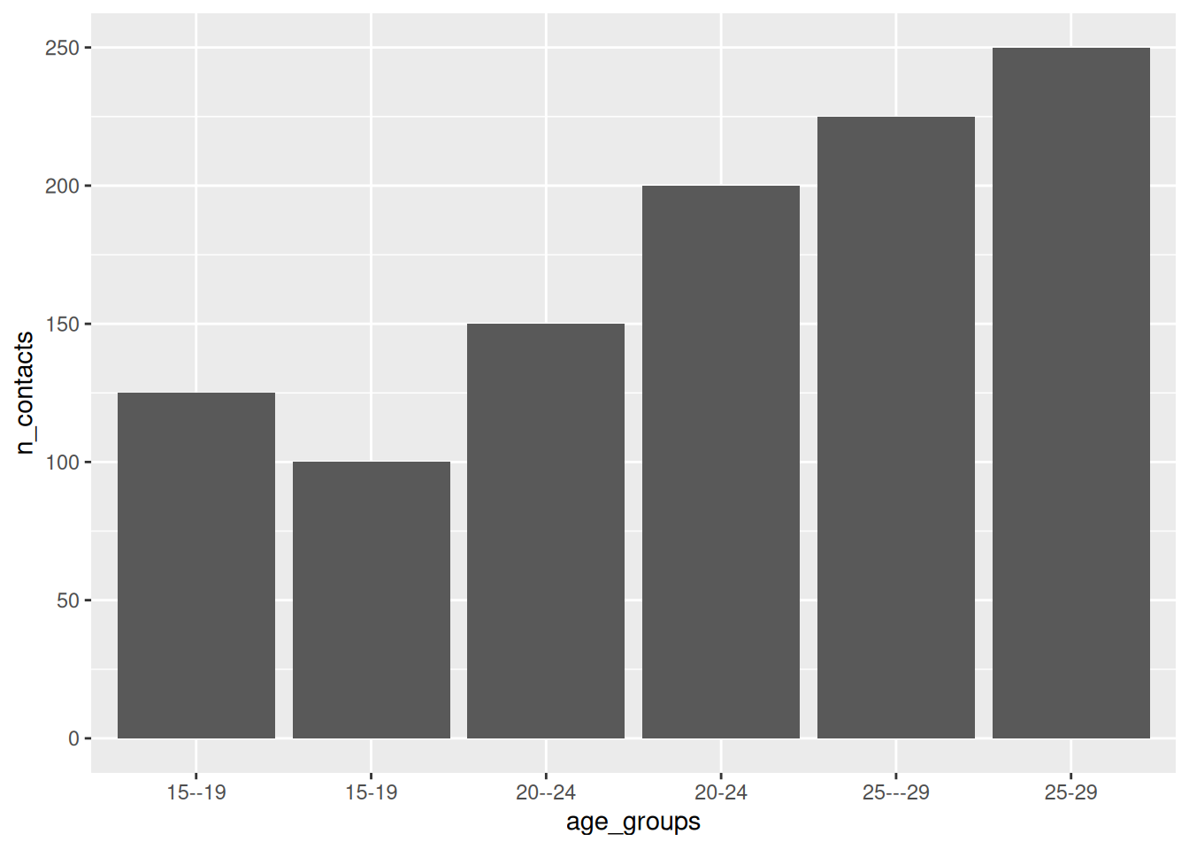
Let’s say we had some data on age groups - the number of contacts these people record on a given day.

options(tidyverse.quiet=TRUE)
library(tidyverse)
contact <- tibble(
  location = rep(c("QLD", "NSW"), 3),
  age_groups = c("15-19", "15--19", "20--24", "20-24", "25---29", "25-29"),
  n_contacts = c(100, 125, 150, 200, 225, 250)
)

contact

# A tibble: 6 × 3
  location age_groups n_contacts
  <chr>    <chr>           <dbl>
1 QLD      15-19             100
2 NSW      15--19            125
3 QLD      20--24            150
4 NSW      20-24             200
5 QLD      25---29           225
6 NSW      25-29             250

We want to produce a plot of age groups and the number of contacts.

But, we can’t do this, because there are all these different ways of representing “age_group”.

ggplot(
  contact,
  aes(x = age_groups,
      y = n_contacts)) + 
  geom_col()

Well rather, we CAN do this, but we want to get the totals of each age group.

What we want out of this is them all to be separated out by an underscore “_“, and turned into a factor:

library(stringr)
tidy_contact <- contact |> 
  mutate(
    age_groups = str_replace_all(
      string = age_groups, 
      pattern = "---|--|-",
      replacement = "_"
      ),
    age_groups = as.factor(age_groups)
  )

tidy_contact

# A tibble: 6 × 3
  location age_groups n_contacts
  <chr>    <fct>           <dbl>
1 QLD      15_19             100
2 NSW      15_19             125
3 QLD      20_24             150
4 NSW      20_24             200
5 QLD      25_29             225
6 NSW      25_29             250

And then we can plot this:

ggplot(
  tidy_contact,
  aes(x = age_groups,
      y = n_contacts)) + 
  geom_col()

Sure, job done.

But now we have some new data, this one contains similar information, but it has population data that we need to join onto it so we can get proportion information.

population <- tibble(
  location = rep(c("QLD", "NSW"), 3),
  age_groups = c("15--19", "15-19", "20---24", "20-24", "25-29", "25--29"),
  population = c(319014, 468550, 338824, 540233, 370468, 607891)
)

population

# A tibble: 6 × 3
  location age_groups population
  <chr>    <chr>           <dbl>
1 QLD      15--19         319014
2 NSW      15-19          468550
3 QLD      20---24        338824
4 NSW      20-24          540233
5 QLD      25-29          370468
6 NSW      25--29         607891

And this is why I think you should write a function.

We want to encapsulate the idea of cleaning up age group. That is: “clean age groups”. So let’s write a function that captures this idea.

clean_age_groups <- function(age_groups){
  
  age_underscore <- str_replace_all(
      string = age_groups, 
      pattern = "---|--|-",
      replacement = "_"
      )
  as.factor(age_underscore)
  
}

And this is the difference in the worflow, for each of these, script, or function tidying up processes:

script
function

tidy_contact <- contact |> 
  mutate(
    age_groups = str_replace_all(
      string = age_groups, 
      pattern = "---|--|-",
      replacement = "_"
      ),
    age_groups = as.factor(age_groups)
  )

tidy_population <- population |> 
  mutate(
    age_groups = str_replace_all(
      string = age_groups, 
      pattern = "---|--|-",
      replacement = "_"
      ),
    age_groups = as.factor(age_groups)
  )

tidy_proportion <- tidy_contact |> 
  left_join(tidy_population,
             by = c("location", "age_groups")) |> 
  mutate(proportion = n_contacts / population)
  

tidy_proportion

# A tibble: 6 × 5
  location age_groups n_contacts population proportion
  <chr>    <fct>           <dbl>      <dbl>      <dbl>
1 QLD      15_19             100     319014   0.000313
2 NSW      15_19             125     468550   0.000267
3 QLD      20_24             150     338824   0.000443
4 NSW      20_24             200     540233   0.000370
5 QLD      25_29             225     370468   0.000607
6 NSW      25_29             250     607891   0.000411

clean_age_groups <- function(age_groups){
  
  age_underscore <- str_replace_all(
      string = age_groups, 
      pattern = "---|--|-",
      replacement = "_"
      )
  as.factor(age_underscore)
  
}

tidy_contact <- contact |> 
  mutate(
    age_groups = clean_age_groups(age_groups)
  )

tidy_population <- population |> 
  mutate(
    age_groups = clean_age_groups(age_groups)
  )

tidy_proportion <- tidy_contact |> 
  left_join(tidy_population,
             by = c("location", "age_groups")) |> 
  mutate(proportion = n_contacts / population)

5.6.1 Functions give ideas a home

Functions provide a way to express the idea of what we want to do. They also provide your ideas a home. What if the data changes? Do you want to go back and change each line of code? No! You can update the function in one place, and then repeat it again.

Once you start writing functions to do things, they will start to be little repositories of knowledge. Little shortcuts that you can use to just remember the most important part.

Now, on to the anatomy of functions

5.7 Anatomy of a function

Now, to speak about the mechanics of writing functions: a function is composed of three parts:

Name
Arguments
Body

To look at our clean_age_groups function again, we can see the following:

# The name of the function
clean_age_groups <- function(age_groups){ # The argument - age_groups
  
  # The body of the function
  age_underscore <- str_replace_all(
      string = age_groups, 
      pattern = "---|--|-",
      replacement = "_"
      )
  
  # The last thing you do with the function is what it returns
  as.factor(age_underscore)
  
}

The last thing you do shouldn’t be assignment <-

The last thing that a function does is what it returns. If we take our example above and change the last line to assign to some variable, then the function will not return anything!

# The name of the function
clean_age_groups <- function(age_groups){ # The argument - age_groups
  
  # The body of the function
  age_underscore <- str_replace_all(
      string = age_groups, 
      pattern = "---|--|-",
      replacement = "_"
      )
  
  # The last thing you do with the function is what it returns
  factored <- as.factor(age_underscore)
  
}

clean_age_groups("10--11")

This is a pretty common mistake, one I still make–something to be aware of!

The way to fix this is to make sure that the last thing you do isn’t assigned. So, our example above should look like so:

# The name of the function
clean_age_groups <- function(age_groups){ # The argument - age_groups
  
  # The body of the function
  age_underscore <- str_replace_all(
      string = age_groups, 
      pattern = "---|--|-",
      replacement = "_"
      )
  
  # The last thing you do with the function is what it returns
  # NOT THIS
  # factored <- as.factor(age_underscore)
  # THIS
  as.factor(age_underscore)
  
}

clean_age_groups("10--11")

[1] 10_11
Levels: 10_11

5.8 How to think about writing functions

There are many ways to start writing functions.

Fundamentally, it is about identifying inputs and outputs.

One useful approach, I think, is to identify the outputs before the inputs:

The output. What one thing do you want this function to return?
The input. What (potentially many) thing(s) go in to this.

This “gestalt”, or top-down approach isn’t how it always needs to be done. But I think it helps you identify the thing you need first, which can help guide you.

5.8.1 Identifying the output - what do we need?

It might feel a bit like putting the cart before the horse, but I think there is a nice advantage to thinking about the output first: you focus on what you want the function to do.

In the case of our clean_age_groups function, we want to get values like “15_19” that are factors.

5.8.2 Identifying the input

So now we have a clear idea of what we need - we can now clarify what we have, which in our case earlier, was some contact data

contact

# A tibble: 6 × 3
  location age_groups n_contacts
  <chr>    <chr>           <dbl>
1 QLD      15-19             100
2 NSW      15--19            125
3 QLD      20--24            150
4 NSW      20-24             200
5 QLD      25---29           225
6 NSW      25-29             250

Where we want to focus on age groups, and take inputs like

c("15-19", "15--19")

[1] "15-19"  "15--19"

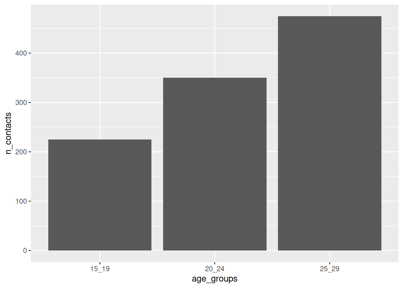
And then turn them into:

c("15_19", "15_19")

[1] "15_19" "15_19"

Breaking things down like this means we can focus on a really small example of the thing we want, which makes the problem easier to solve.

There are many ways to manage turning strings into other strings, and I like to use the stringr package to do this. We can use the str_replace_all function. So I’ll start by scratching up some inputs like so, and seeing if this works

ages <- c("15-19", "15--19")
str_replace_all(
  string = ages,
  pattern = "-",
  replacement = "_"
)

[1] "15_19"  "15__19"

Not quite what I’m after - I’ve got two underscores when I want just one.

5.8.2.1 Iteration: Writing functions is writing

I didn’t get this right the first time - and I rarely do! The point I want to make here is:

Writing functions is just like writing. It takes iteration.

We have incidentally replaced every - with _, which means -- becomes __.

Let’s change that by using | in the “pattern” argument, which allows us to specify -|--, which means, - OR --:

ages <- c("15-19", "15--19")
str_replace_all(
  string = ages,
  pattern = "-|--",
  replacement = "_"
)

[1] "15_19"  "15__19"

OK, the same problem. We actually need to flip the order here, so we change -- first:

ages <- c("15-19", "15--19")
str_replace_all(
  string = ages,
  pattern = "--|-",
  replacement = "_"
)

[1] "15_19" "15_19"

Great! Now let’s put that into the body of the function, and give the function a good name.

clean_age_groups <- function(age_groups){
  str_replace_all(
  string = ages,
  pattern = "--|-",
  replacement = "_"
)
}

clean_age_groups(ages)

[1] "15_19" "15_19"

It’s a useful process to scratch out a function like this. As you get more confident with this, you will start to be able to write the code as a function first, and then iterate in that way.

beware copying and pasting into functions

The process of writing a function out in scratchings as we’ve done, is that we can leave some scraps in the code. In this case, I’ve actually left the ages object in the function, but the argument is age_groups:

clean_age_groups <- function(age_groups){
  str_replace_all(
  string = ages,
  pattern = "--|-",
  replacement = "_"
)
}

clean_age_groups(ages)

[1] "15_19" "15_19"

Notice that this still works! This is because the ages object still exists as a variable I’ve created. But if we try another input, we’ll get some strange output:

clean_age_groups(c("10-12", "10--12"))

[1] "15_19" "15_19"

So, make sure to clean up after you’ve copied and pasted - remember to check the arguments match how they are used in the function.

And on that note, let’s redefine clean_age_groups correctly so we don’t get an error later on (which happened during the development of the book)

clean_age_groups <- function(age_groups){
  str_replace_all(
  string = age_groups,
  pattern = "--|-",
  replacement = "_"
)
}

clean_age_groups(ages)

[1] "15_19" "15_19"

5.8.3 Managing scope - functions are best (generally) when they do one thing

Also, note that we wrote clean_age_groups to just focus on converting input like “10–12” into “10_12”. We could have instead focussed on cleaning up the data frame, like so:

contact

# A tibble: 6 × 3
  location age_groups n_contacts
  <chr>    <chr>           <dbl>
1 QLD      15-19             100
2 NSW      15--19            125
3 QLD      20--24            150
4 NSW      20-24             200
5 QLD      25---29           225
6 NSW      25-29             250

clean_age_groups_data <- function(data){
  
  tidy_contact <- data |> 
  mutate(
    age_groups = str_replace_all(
      string = age_groups, 
      pattern = "---|--|-",
      replacement = "_"
      ),
    age_groups = as.factor(age_groups)
  )
  
  tidy_contact

}

clean_age_groups_data(contact)

# A tibble: 6 × 3
  location age_groups n_contacts
  <chr>    <fct>           <dbl>
1 QLD      15_19             100
2 NSW      15_19             125
3 QLD      20_24             150
4 NSW      20_24             200
5 QLD      25_29             225
6 NSW      25_29             250

I think there are a couple of issues with this:

We assume the age groups column is always age_groups
The scope is now larger - we are always working with data and returning data
We haven’t necessarily made the expression easier.

It is fine to wrap up the existing function into another function that cleans the data - to me this better encapsulates and expresses the ideas:

contact

# A tibble: 6 × 3
  location age_groups n_contacts
  <chr>    <chr>           <dbl>
1 QLD      15-19             100
2 NSW      15--19            125
3 QLD      20--24            150
4 NSW      20-24             200
5 QLD      25---29           225
6 NSW      25-29             250

clean_contacts <- function(data){
  
  data |> 
  mutate(
    age_groups = clean_age_groups(age_groups)
  )

}

clean_contacts(contact)

# A tibble: 6 × 3
  location age_groups n_contacts
  <chr>    <chr>           <dbl>
1 QLD      15_19             100
2 NSW      15_19             125
3 QLD      20_24             150
4 NSW      20_24             200
5 QLD      25__29            225
6 NSW      25_29             250

Some of the improvements I notice

We are just focussing on cleaning up the age group column.
We have given it a name that refers to cleaning up the data, which might also give us some space and room to add more cleaning function here.

5.9 When to function

One of my overall points with functions is:

functions help you express your intention.

However, there are some generally good heuristics to follow to help guide you towards writing a function. Generally, it is time to write a function if:

You’ve copied and pasted the code 3 or more times.
You’ve re-read your code more than 3 times.

This first principle is often called DRY - “Don’t Repeat Yourself.

The second principle has been coined by Miles McBain, also as DRY, or possibly DRRY: Don’t ReRead Yourself.

5.10 Naming things is hard

There are only two hard things in Computer Science: cache invalidation and naming things.

– Phil Karlton

What does this function do?

myfun <- function(x){
  (x * 9/5) + 32
}

Converting temperature?

temperature_conversion <- function(x){
  (x * 9/5) + 32
}

Clearly state input_to_output()

celcius_to_fahrenheit <- function(x){
  (x * 9/5) + 32
}

Name argument and intermediate variables

celcius_to_fahrenheit <- function(celcius){
  fahrenheit <- (celcius * 9/5) + 32
  fahrenheit
}

What, what does make functions hard?

celcius_to_fahrenheit <- function(celcius){
  (celcius * 9/5) + 32
}

Identifying inputs and outputs is hard.

But what is hard it taking code, (like the code in a data analysis) and finding the parts that need to change

There’s a level of “I got it to work” and there’s a level of “It works, and I can reason about it”

– Joe Cheng You have to be able to reason about it | Data Science Hangout

I can reason about it

…how do you take all this complexity and break it down into smaller pieces…each of which you can reason about…each of which you can hold in your head…each of which you can look at and be like “yup, I can fully ingest this entire function definition, I can read it line by line and prove to myself this is definitely correct…So software engineering… is a lot about this: How do you break up inherently complicated things that we are trying to do into small pieces that are individually easy to reason about. That’s half the battle…The other half of the battle is how do we combine them in ways that can be reliable and also easy to reason about

5.11 The other hard part of writing functions

Practice naming things

Give names to the following functions:

thingy <- function(x){
  x^3
}

bobby <- function(x){
  str_replace_all(
    string = x,
    pattern = "“",
    replacement = '"'
  )
}

f <- function(x) {
  ux <- unique(x)
  ux[which.max(tabulate(match(x, ux)))]
}

Generally speaking, it is good to following a naming convention of some kind, and also to keep the names descriptive:

# good
fit_lm()
fit_cart()
fit_glm()

# less good - tab complete isn't as good, unless we have a lot of functions also named `lm` and `cart`, and `glm`. We don't emphasize things
lm_fit()
cart_fit()
glm_fit()

# bad
flm()
fcart()
fglm()

5.12 Conclusion

The process of writing a function is:

Identify outputs and inputs
Identify the complexity to abstract away
Writing functions is iterative, Just like regular writing
Naming things is hard. Focus on making “slightly better” names.

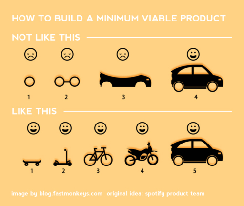
On a final note, I think it’s worthwhile thinking about the iteration - and the idea of moving from a skateboard to a car, rather than building the car:

(heard via Stat545 functions chapter)